SPARK재설치

일시 : 10.02

대상서버 : bigdata07, 08, 09, 10

JDK 설치

jdk version

파일 다운로드

jdk 파일 다운로드 및 설치 할 서버로 업로드.

  • https://www.oracle.com/technetwork/java/javase/downloads/jdk8-downloads-2133151.html

설치 경로에 다운로드 받은 파일 압축 해제

  • /usr/lib/jvm

심볼릭 링크 설정

기존 자바의 심볼릭 링크 삭제

java 명령은 /usr/bin/java 또는 javac의 심볼릭 링크이다.

etc/alternateives 경로 아래에 있는 java 혹은 javac의 심볼릭 링크를 삭제 한다.

rm  /etc/alternatives/java
# rm  /etc/alternatives/javac

새로 다운로드 받은 버전의 경로로 링크 설정

ln -s /usr/lib/jvm/jdk1.8.0_181/bin/java /etc/alternatives/java
# ln -s /usr/lib/jvm/java-1.8.0-openjdk.x86_64/bin/javac /etc/alternatives/javac

JAVA_HOME설정

/etc/profile 또는 ~/.bash_profile등에서 JAVA_HOME 설정.

vi etc/profile

파일 하단에 아래 내용 추가

export JAVA_HOME=/usr/lib/jvm/jdk1.8.0_181
export PATH=$PATH:$JAVA_HOME/bin

scala 설치

설치 scala verseion : 2.12.7

scala 다운로드

다운로드사이트 (https://www.scala-lang.org/download/) 에서 파일 다운로드(rpm 또는 tar.gz)

rpm을 사용해 패키지 설치

rpm -qa scala          # scala 설치 여부 확인
rpm -ivh scala-2.12.7  # scala 설치

SPARK 설치

spark를 클러스터로 동작 시키려면 spark cluster의 자원을 관리 해주는 Cluster manager가 필요하다.

아래의 방법을 사용 할 수 있다.

  • Yarn - hadoop 과 함께 설치.
  • Mesos - 소스코드로 제공되어 운영환경에 맞게 빌드 해주어야 함. gcc 버전 4.8이상.
  • Kubernetes - centos7 이상 사용 가능.
  • Standalone mode

Spark release : 2.3.2

package type : pre-built for apache hadoop 2.7 and later

설치 파일 다운로드

spark 다운로드 페이지 (http://spark.apache.org/downloads.html) 에서 사용할 버전에 맞는 스파크 선택

standalone 설치

참고

  • https://spark.apache.org/docs/latest/spark-standalone.html#installing-spark-standalone-to-a-cluster

설치 정보

master

  • bigdata07.mms.com

slave(worker)

  • bigdata07.mms.com
  • bigdata08.mms.com
  • bigdata09.mms.com
  • bigdata10.mms.com

설치 경로

/usr/local/spark

설정

마스터 서버에서 slave정보를 입력 해줘야함.

slave로 사용할 서버에 spark 설치 해야 한다.

실행

master구동

마스터 서버에서 $SPARK_HOME/sbin/start-master.sh 스크립트를 실행.

마스터를 실행하게 되면 데몬으로 동작하며 spark_master_url:8080에 웹서버가 구동되므로 페이지에 접근이 가능하면 정상적으로 구동된 것이다.

slave 구동

각 slave 노드에서 $SPARK_HOME/sbin/start-slave.sh스크립트를 사용해 worker를 구동 시켜야 한다.

$SPARK_HOME/sbin/start-slave.sh spark_master_url:spark_port

스파크 마스터가 7077에서 구동되므로 ./start-slave.sh bigdata07.mms.com:7077 커맨드로 실행한다.

정상적으로 작동이 되면 master의 UI 페이지에서 확인이 가능하다.

테스트

spark-submit을 이용해 테스트

$ ./spark-submit \
     --master spark://192.168.100.17:7077 \
     --class org.apache.spark.examples.SparkPi \
     /usr/local/spark/examples/jars/spark-examples*.jar \
     100


분석서버 현황

Host name
Application
추가 설치 안
bigdata01zookeeper
bigdata02zookeeper
bigdata03kafka
bigdata04kafka
bigdata05kafka
bigdata06zookeeper
bigdata07spark
bigdata08spark
bigdata09spark
bigdata10spark
bigdata11ML
bigdata12
kafka
bigdata13
kafka
bigdata14
spark
bigdata15Yum Repospark


Kafka, Spark 처리 결과

-test1

input size : 1.4T 모든서버

conditions : watermark 60s, trigger 1s

Test time : 10am~1pm

result : 오답률 50%이상

오답 원인 : 1차 ETL 병목 현상 (3번 Kafka 서버 특정 파티션 consumer 지연)


-test2 

input size : 1.4T 모든서버

Conditions : watermark 120s, trigger 2s , 3,4,5 번 서버 Thread 옵션 조정 (8,8,8 → 6,9,9)

Test time : 2pm~3pm

result : 오답률 1% 이하


* spark watermark (지연시간) 를 줄이고 오답률을 개선하려면,

KAFKA /SPARK 클러스터를 복합적으로 늘려서

KAFKA 파티션 , SPARK RDD 파티션, Spark core수 , 1차 ETL 병목 현상

등 복합적으로 개선이 되어야 합니다.

Log Data 분석 시간 결과

-

분석 서버 부하 결과(CPU, Mmemory, Disk I/O)

CPU, Memory, Disk I/O 사용률 - 요약

buffer cache flush 필요

Host name
CPU(%user)
Memory
Disk I/O
buffer cach flush
bigdata010.26%10%
10.56%
bigdata020.16%31%
5.83%
bigdata0345%99%
15%
bigdata0455%99%
12.4%
bigdata0545%99%
10.7%
bigdata060.2%81%
5%
bigdata0718%99%
8%
bigdata0818%99%
12.4%
bigdata0917%99%
10.9%
bigdata1015%99%
11.8%
bigdata111.5%99%
7%
bigdata1211%99%
35.8%
bigdata133%99%
22%
bigdata141%99%
5.7%
bigdata151.5%99%
8%


Query Type
Supported Output ModesNotes
Queries with aggregationAggregation on event-time with watermarkAppend, Update, CompleteAppend mode uses watermark to drop old aggregation state. But the output of a windowed aggregation is delayed the late threshold specified in `withWatermark()` as by the modes semantics, rows can be added to the Result Table only once after they are finalized (i.e. after watermark is crossed). See the Late Data section for more details. 

Update mode uses watermark to drop old aggregation state. 

Complete mode does not drop old aggregation state since by definition this mode preserves all data in the Result Table.
Other aggregationsComplete, UpdateSince no watermark is defined (only defined in other category), old aggregation state is not dropped. 

Append mode is not supported as aggregates can update thus violating the semantics of this mode.
Queries with mapGroupsWithStateUpdate
Queries with flatMapGroupsWithStateAppend operation modeAppendAggregations are allowed after flatMapGroupsWithState.
Update operation modeUpdateAggregations not allowed after flatMapGroupsWithState.
Queries with joinsAppendUpdate and Complete mode not supported yet. See the support matrix in the Join Operations section for more details on what types of joins are supported.
Other queriesAppend, UpdateComplete mode not supported as it is infeasible to keep all unaggregated data in the Result Table.


Output Sinks

There are a few types of built-in output sinks.

  • File sink - Stores the output to a directory.

    writeStream
        .format("parquet")        // can be "orc", "json", "csv", etc.
        .option("path""path/to/destination/dir")
        .start()


  • Kafka sink - Stores the output to one or more topics in Kafka.

    writeStream
        .format("kafka")
        .option("kafka.bootstrap.servers""host1:port1,host2:port2")
        .option("topic""updates")
        .start()


  • Foreach sink - Runs arbitrary computation on the records in the output. See later in the section for more details.

    writeStream
        .foreach(...)
        .start()


  • Console sink(for debugging) - Prints the output to the console/stdout every time there is a trigger. Both, Append and Complete output modes, are supported. This should be used for debugging purposes on low data volumes as the entire output is collected and stored in the driver’s memory after every trigger.

    writeStream
        .format("console")
        .start()


  • Memory sink (for debugging) - The output is stored in memory as an in-memory table. Both, Append and Complete output modes, are supported. This should be used for debugging purposes on low data volumes as the entire output is collected and stored in the driver’s memory. Hence, use it with caution.

    writeStream
        .format("memory")
        .queryName("tableName")
        .start()


Some sinks are not fault-tolerant because they do not guarantee persistence of the output and are meant for debugging purposes only. See the earlier section on fault-tolerance semantics. Here are the details of all the sinks in Spark.

Sink
Supported Output Modes
Options
Fault-tolerant
Notes
File SinkAppendpath: path to the output directory, must be specified. 

For file-format-specific options, see the related methods in DataFrameWriter (Scala/Java/Python/R). E.g. for "parquet" format options see DataFrameWriter.parquet()
Yes (exactly-once)Supports writes to partitioned tables. Partitioning by time may be useful.
Kafka SinkAppend, Update, CompleteSee the Kafka Integration GuideYes (at-least-once)More details in the Kafka Integration Guide
Foreach SinkAppend, Update, CompleteNoneDepends on ForeachWriter implementationMore details in the next section
Console SinkAppend, Update, CompletenumRows: Number of rows to print every trigger (default: 20) 
truncate: Whether to truncate the output if too long (default: true)
No
Memory SinkAppend, CompleteNoneNo. But in Complete Mode, restarted query will recreate the full table.Table name is the query name.


'spark,kafka,hadoop ecosystems > apache spark' 카테고리의 다른 글

spark 재설치  (0) 2018.11.21
etl 통테 결과  (0) 2018.11.21
Spark Struct Streaming - joins  (0) 2018.11.20
Spark Struct Streaming - other operations  (0) 2018.11.20
spark struct streaming - window operation  (0) 2018.11.20

2.3.0 부터 지원된다.,

(IPC - 2.2.0 , EPC 2.3.0)

Support matrix for joins in streaming queries
Left InputRight InputJoin Type
StaticStaticAll typesSupported, since its not on streaming data even though it can be present in a streaming query
StreamStaticInnerSupported, not stateful
Left OuterSupported, not stateful
Right OuterNot supported
Full OuterNot supported
StaticStreamInnerSupported, not stateful
Left OuterNot supported
Right OuterSupported, not stateful
Full OuterNot supported
StreamStreamInnerSupported, optionally specify watermark on both sides + time constraints for state cleanup
Left OuterConditionally supported, must specify watermark on right + time constraints for correct results, optionally specify watermark on left for all state cleanup
Right OuterConditionally supported, must specify watermark on left + time constraints for correct results, optionally specify watermark on right for all state cleanup
Full OuterNot supported
import org.apache.spark.sql.functions.expr
 
val impressions = spark.readStream. ...
val clicks = spark.readStream. ...
 
// Apply watermarks on event-time columns
val impressionsWithWatermark = impressions.withWatermark("impressionTime""2 hours")
val clicksWithWatermark = clicks.withWatermark("clickTime""3 hours")
 
// Join with event-time constraints
impressionsWithWatermark.join(
  clicksWithWatermark,
  expr("""
    clickAdId = impressionAdId AND
    clickTime >= impressionTime AND
    clickTime <= impressionTime + interval 1 hour
    """)
)
 
 
impressionsWithWatermark.join(
  clicksWithWatermark,
  expr("""
    clickAdId = impressionAdId AND
    clickTime >= impressionTime AND
    clickTime <= impressionTime + interval 1 hour
    """),
  joinType = "leftOuter"      // can be "inner", "leftOuter", "rightOuter"
 )


정리하자면, STREAM - STREAM JOIN 에서 INNER 조인은 watermark 가 옵셔날이지만 의미적으로도 써주는것이 좋고 성능도개선된다.

OUTER 조인은 Watermark 가 필수인데 ,그이유는 마지막까지 조인할 대상을 찾고 기다리기 때문에,  만약 null 일 경우 delay time 은 최대가된다.


  • Joins can be cascaded, that is, you can do df1.join(df2, ...).join(df3, ...).join(df4, ....).

  • As of Spark 2.3, you can use joins only when the query is in Append output mode. Other output modes are not yet supported.

  • As of Spark 2.3, you cannot use other non-map-like operations before joins. Here are a few examples of what cannot be used.

    • Cannot use streaming aggregations before joins.

    • Cannot use mapGroupsWithState and flatMapGroupsWithState in Update mode before joins.


  1. deduplication

    / Without watermark using guid column
    streamingDf.dropDuplicates("guid")
     
    // With watermark using guid and eventTime columns
    streamingDf
      .withWatermark("eventTime""10 seconds")
      .dropDuplicates("guid""eventTime")

    watermark - watermark 까지 (참고로 이전 date 는 중복제거가 안 될 수 있음)
    without - sate 되는대까지

  2. Arbitary State
    Since Spark 2.2, this can be done using the operation mapGroupsWithState and the more powerful operation flatMapGroupsWithState. Both operations allow you to apply user-defined code on grouped Datasets to update user-defined state. For more concrete details, take a look at the API documentation (Scala/Java) and the examples (Scala/Java).
    위의 Operation 은 유저가원하는(임의의) state 를 만든다. 다만 그 State 가 어떻게 활용되는지는 별이야기가없다.

     3. Unsupported!

Unsupported Operations

There are a few DataFrame/Dataset operations that are not supported with streaming DataFrames/Datasets. Some of them are as follows.

  • Multiple streaming aggregations (i.e. a chain of aggregations on a streaming DF) are not yet supported on streaming Datasets.

  • Limit and take first N rows are not supported on streaming Datasets.

  • Distinct operations on streaming Datasets are not supported.

  • Sorting operations are supported on streaming Datasets only after an aggregation and in Complete Output Mode.

  • Few types of outer joins on streaming Datasets are not supported. See the support matrix in the Join Operations section for more details.

In addition, there are some Dataset methods that will not work on streaming Datasets. They are actions that will immediately run queries and return results, which does not make sense on a streaming Dataset. Rather, those functionalities can be done by explicitly starting a streaming query (see the next section regarding that).

  • count() - Cannot return a single count from a streaming Dataset. Instead, use ds.groupBy().count() which returns a streaming Dataset containing a running count.

  • foreach() - Instead use ds.writeStream.foreach(...) (see next section).

  • show() - Instead use the console sink (see next section).


val query = df.writeStream.format("console").start()   // get the query object
 
query.id          // get the unique identifier of the running query that persists across restarts from checkpoint data
 
query.runId       // get the unique id of this run of the query, which will be generated at every start/restart
 
query.name        // get the name of the auto-generated or user-specified name
 
query.explain()   // print detailed explanations of the query
 
query.stop()      // stop the query
 
query.awaitTermination()   // block until query is terminated, with stop() or with error
 
query.exception       // the exception if the query has been terminated with error
 
query.recentProgress  // an array of the most recent progress updates for this query
 
query.lastProgress    // the most recent progress update of this streaming query


val spark: SparkSession = ...
 
spark.streams.active    // get the list of currently active streaming queries
 
spark.streams.get(id)   // get a query object by its unique id
 
spark.streams.awaitAnyTermination()   // block until any one of them terminates


Window Operations on Event Time

Aggregations over a sliding event-time window are straightforward with Structured Streaming and are very similar to grouped aggregations. In a grouped aggregation, aggregate values (e.g. counts) are maintained for each unique value in the user-specified grouping column. In case of window-based aggregations, aggregate values are maintained for each window the event-time of a row falls into. Let’s understand this with an illustration.

>>Aggeregation 과정은 Structured Streaming 에서 똑바르며 grouped aggregation 과 유사하다. 다만 grouped aggregation 에서는 특정컬럼을 기준으로 정리되는데 window - based aggregation 은 Event time 을기준으로 정리된다. 된다.

Imagine our quick example is modified and the stream now contains lines along with the time when the line was generated. Instead of running word counts, we want to count words within 10 minute windows, updating every 5 minutes. That is, word counts in words received between 10 minute windows 12:00 - 12:10, 12:05 - 12:15, 12:10 - 12:20, etc. Note that 12:00 - 12:10 means data that arrived after 12:00 but before 12:10. Now, consider a word that was received at 12:07. This word should increment the counts corresponding to two windows 12:00 - 12:10 and 12:05 - 12:15. So the counts will be indexed by both, the grouping key (i.e. the word) and the window (can be calculated from the event-time).

The result tables would look something like the following.

Window Operations

`Furthermore, this model naturally handles data that has arrived later than expected based on its event-time. Since Spark is updating the Result Table, it has full control over updating old aggregates when there is late data, as well as cleaning up old aggregates to limit the size of intermediate state data. Since Spark 2.1, we have support for watermarking which allows the user to specify the threshold of late data, and allows the engine to accordingly clean up old state. These are explained later in more detail in the Window Operations section.

>> 기본적으로 늦은 data 들에 대해서 처리를 하지만, Spark 는 늦은데이타에서 업데이트를 지속하기위해서 old value 를 컨트롤한다. 뿐만아니라 cleaning up 도한다.

2.1 에서부터는 watermarking 을 제공하여 늦은데이타를 날릴 수 있는 Threshold 값을 조절 할 수 있다.


Now consider what happens if one of the events arrives late to the application. For example, say, a word generated at 12:04 (i.e. event time) could be received by the application at 12:11. The application should use the time 12:04 instead of 12:11 to update the older counts for the window 12:00 - 12:10. This occurs naturally in our window-based grouping – Structured Streaming can maintain the intermediate state for partial aggregates for a long period of time such that late data can update aggregates of old windows correctly, as illustrated below.z`Handling Late Data

However, to run this query for days, it’s necessary for the system to bound the amount of intermediate in-memory state it accumulates. This means the system needs to know when an old aggregate can be dropped from the in-memory state because the application is not going to receive late data for that aggregate any more. To enable this, in Spark 2.1, we have introduced watermarking, which lets the engine automatically track the current event time in the data and attempt to clean up old state accordingly. You can define the watermark of a query by specifying the event time column and the threshold on how late the data is expected to be in terms of event time. For a specific window starting at time T, the engine will maintain state and allow late data to update the state until (max event time seen by the engine - late threshold > T). In other words, late data within the threshold will be aggregated, but data later than the threshold will start getting dropped (see later in the section for the exact guarantees). Let’s understand this with an example. We can easily define watermarking on the previous example using withWatermark() as shown below.

>>하지만 이것을 일단위로 돌리려면, state data 를 memory 에 들어야하고, 블라블라~ water marking 써야하고 > 이것이 지속적인 성능을 향상

import spark.implicits._
 
val words = ... // streaming DataFrame of schema { timestamp: Timestamp, word: String }
 
// Group the data by window and word and compute the count of each group
val windowedCounts = words
    .withWatermark("timestamp""10 minutes")
    .groupBy(
        window($"timestamp""10 minutes""5 minutes"),
        $"word")
    .count()


Watermarking in Update Mode


Watermarking in Append Mode

Similar to the Update Mode earlier, the engine maintains intermediate counts for each window. However, the partial counts are not updated to the Result Table and not written to sink. The engine waits for “10 mins” for late date to be counted, then drops intermediate state of a window < watermark, and appends the final counts to the Result Table/sink. For example, the final counts of window 12:00 - 12:10 is appended to the Result Table only after the watermark is updated to 12:11.

>> Append mode 의경우 watermark 의 유효기간까지 data 를 유지하고, 유효기간이 완료되면 추가된 row 들만 append 하게된다.


Conditions for watermarking to clean aggregation state

watermarking을 하기 위해선 아래조건이 만족 필요

  • Output mode must be Append or Update. Complete mode requires all aggregate data to be preserved, and hence cannot use watermarking to drop intermediate state. See the Output Modes section for detailed explanation of the semantics of each output mode.

  • The aggregation must have either the event-time column, or a window on the event-time column.

  • withWatermark must be called on the same column as the timestamp column used in the aggregate. For example, df.withWatermark("time", "1 min").groupBy("time2").count() is invalid in Append output mode, as watermark is defined on a different column from the aggregation column.

  • withWatermark must be called before the aggregation for the watermark details to be used. For example, df.groupBy("time").count().withWatermark("time", "1 min") is invalid in Append output mode.


Semantic Guarantees of Aggregation with Watermarking
  • A watermark delay (set with withWatermark) of “2 hours” guarantees that the engine will never drop any data that is less than 2 hours delayed. In other words, any data less than 2 hours behind (in terms of event-time) the latest data processed till then is guaranteed to be aggregated.

  • However, the guarantee is strict only in one direction. Data delayed by more than 2 hours is not guaranteed to be dropped; it may or may not get aggregated. More delayed is the data, less likely is the engine going to process it.


Programming Model

The key idea in Structured Streaming is to treat a live data stream as a table that is being continuously appended. This leads to a new stream processing model that is very similar to a batch processing model. You will express your streaming computation as standard batch-like query as on a static table, and Spark runs it as an incremental query on the unbounded input table. Let’s understand this model in more detail.

> Struct Streaming 의 idea 는  연속된 append 구조이다. 너는 스트리밍 계산을 노말한 batch query 형태로 계산 할 수 있을 것이다.

Basic Concepts

Consider the input data stream as the “Input Table”. Every data item that is arriving on the stream is like a new row being appended to the Input Table.

Stream as a Table

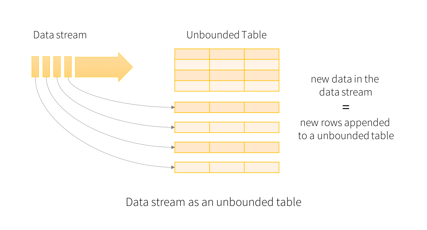
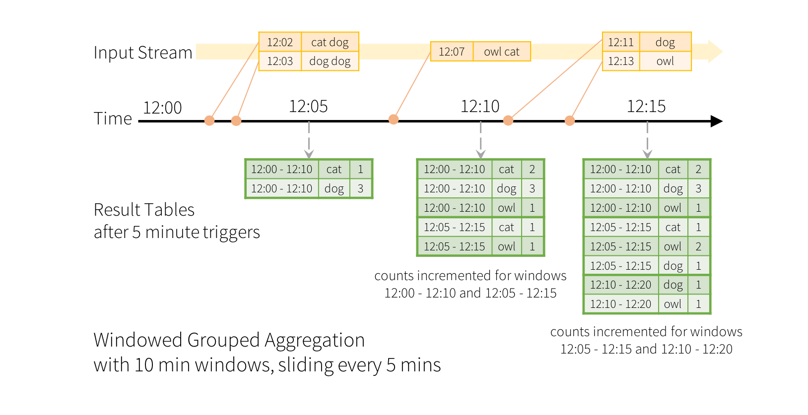
A query on the input will generate the “Result Table”. Every trigger interval (say, every 1 second), new rows get appended to the Input Table, which eventually updates the Result Table. Whenever the result table gets updated, we would want to write the changed result rows to an external sink.

Model

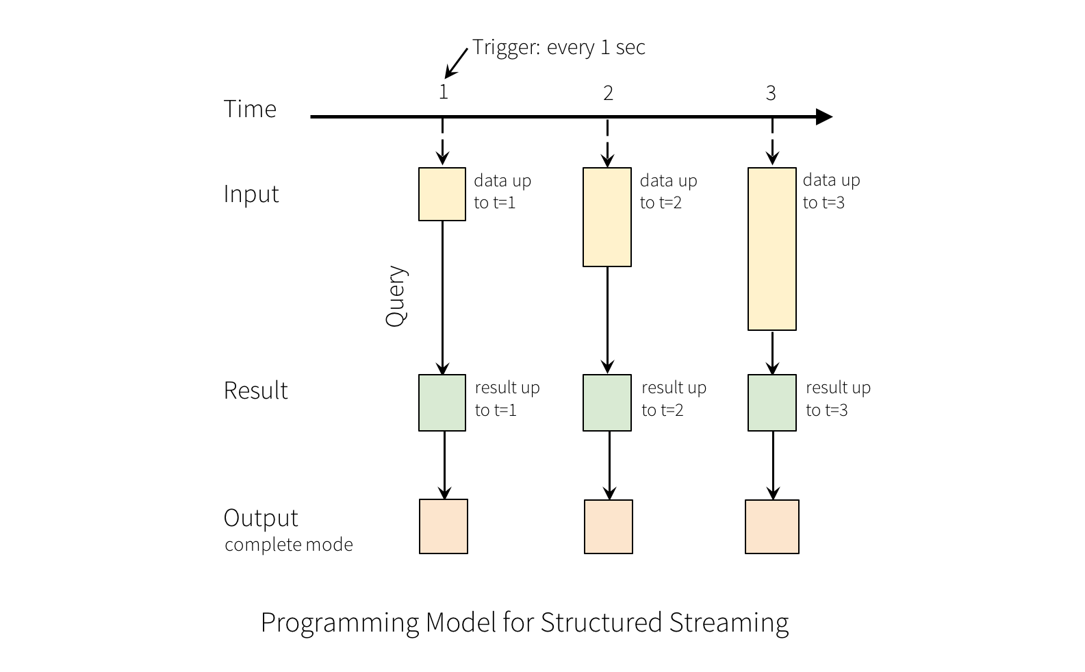
The “Output” is defined as what gets written out to the external storage. The output can be defined in a different mode:

  • Complete Mode - The entire updated Result Table will be written to the external storage. It is up to the storage connector to decide how to handle writing of the entire table.

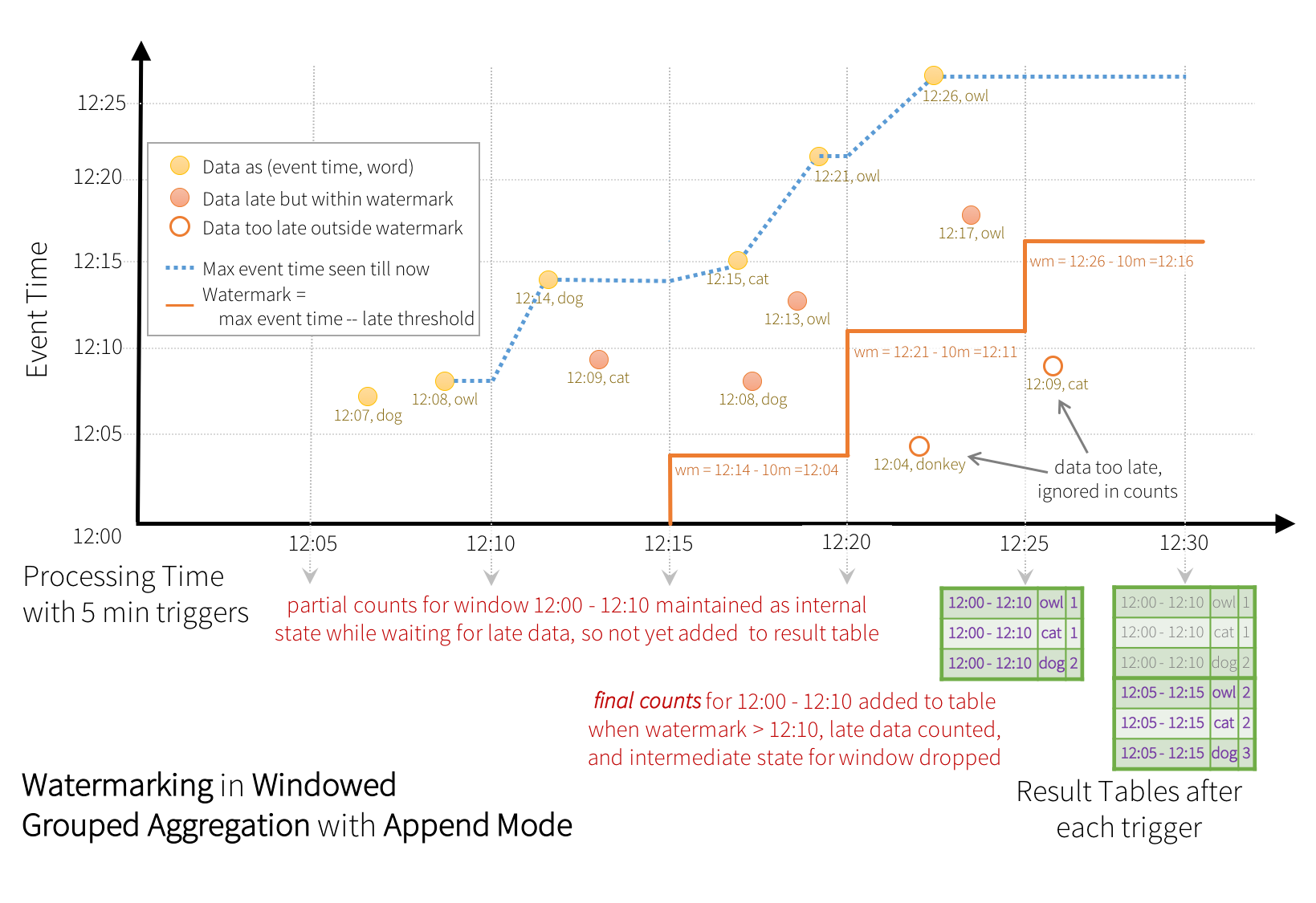
  • Append Mode - Only the new rows appended in the Result Table since the last trigger will be written to the external storage. This is applicable only on the queries where existing rows in the Result Table are not expected to change.

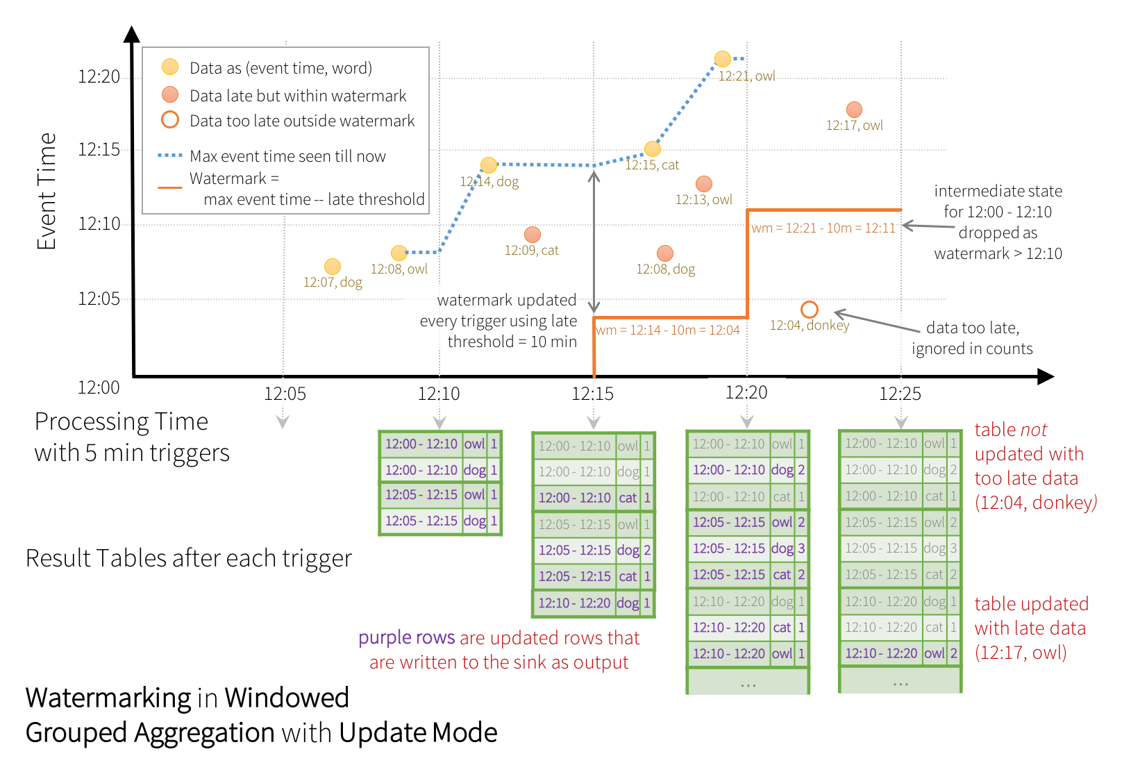
  • Update Mode - Only the rows that were updated in the Result Table since the last trigger will be written to the external storage (available since Spark 2.1.1). Note that this is different from the Complete Mode in that this mode only outputs the rows that have changed since the last trigger. If the query doesn’t contain aggregations, it will be equivalent to Append mode.

Note that each mode is applicable on certain types of queries. This is discussed in detail later.

>> output mode 는 Complete mode / Append mode / Update 모드 3가지 가 있다.

Complete Mode 는 updated 된 Result Table 이 만들어졌을때졌을때,  외부 저장소에 출력된다. 

Append Mode 는 새로운 Rows 들만 Trigger 에 의해 외부저장소에 출력 된다.

Update Mode 란 새롭거나 수정된 Rows 들만 Trigger 에 의해 외부 저장소에 출력 된다. Completed 모드와 다른점은 만약 query 가 Aggregation 을 포함하지 않으면, 이것은 Append Mode 와 똑같이 똑같이 동작한다. (Complete 모드보다 빠를것으로 예상된다.)

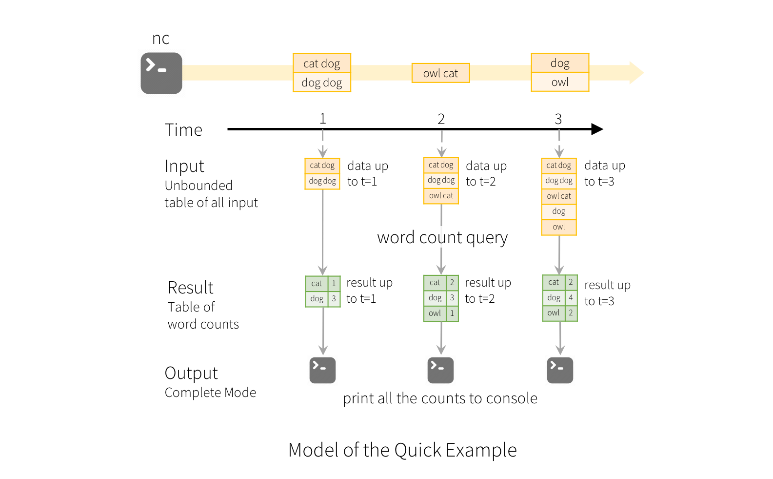
To illustrate the use of this model, let’s understand the model in context of the Quick Example above. The first lines DataFrame is the input table, and the final wordCounts DataFrame is the result table. Note that the query on streaming lines DataFrame to generate wordCounts is exactly the same as it would be a static DataFrame. However, when this query is started, Spark will continuously check for new data from the socket connection. If there is new data, Spark will run an “incremental” query that combines the previous running counts with the new data to compute updated counts, as shown below.

>> 구현하자면  아래와같이 구현한다.

val query = wordCounts.writeStream
.outputMode("complete") or .outputMode("append") or .outputMode("update") 

>>  기존 SQL 과 똑같이 구현하는데, Spark 가 연속적으로 새로운 data 을 체킹한다. (socket 기반) 만약 새로운 Data 가 있으면 Spark 는 증가분에대해서 Query 를 날리게 되고 이전에 돌린 Running count 과 combine 하게 된다. (아래 그림 설명)

Model


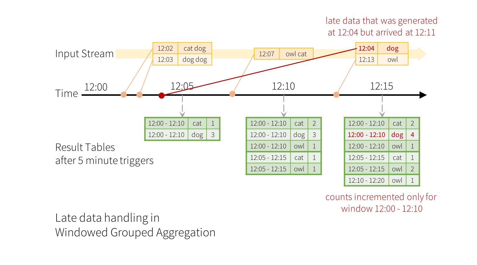
Note that Structured Streaming does not materialize the entire table. It reads the latest available data from the streaming data source, processes it incrementally to update the result, and then discards the source data. It only keeps around the minimal intermediate state data as required to update the result 

>> % Struct Streaming 은 전체 Table 을 구체화 하지 않는다. 그것은 가장 마지막 사용가느한 data 를 읽고 점진적으로 Result 를 update하는 구조이다.

그리고 원본 source data 는 지우게된다. 이것은 가능한 가장 작은 data 를 유지하는데 그것을 state Data 라한다. Result 를 업데이트하기위한 것이 state Data 이기도 하다.

Basic Operations - Selection, Projection, Aggregation

Most of the common operations on DataFrame/Dataset are supported for streaming. The few operations that are not supported are discussed laterin this section.

>> 기본적인 select 등의  Query 를 아래와 같이 지원한다. 다만 몇 몇개는 지원하지 않는다.

case class DeviceData(device: String, deviceType: String, signal: Double, time: DateTime)
 
val df: DataFrame = ... // streaming DataFrame with IOT device data with schema { device: string, deviceType: string, signal: double, time: string }
val ds: Dataset[DeviceData] = df.as[DeviceData]    // streaming Dataset with IOT device data
 
// Select the devices which have signal more than 10
df.select("device").where("signal > 10")      // using untyped APIs
ds.filter(_.signal > 10).map(_.device)         // using typed APIs
 
// Running count of the number of updates for each device type
df.groupBy("deviceType").count()                          // using untyped API
 
// Running average signal for each device type
import org.apache.spark.sql.expressions.scalalang.typed
ds.groupByKey(_.deviceType).agg(typed.avg(_.signal))    // using typed API
Note, you can identify whether a DataFrame/Dataset has streaming data or not by using df.isStreaming.


 unsupported Operation

Schema inference and partition of streaming DataFrames/Datasets

By default, Structured Streaming from file based sources requires you to specify the schema, rather than rely on Spark to infer it automatically. This restriction ensures a consistent schema will be used for the streaming query, even in the case of failures. For ad-hoc use cases, you can reenable schema inference by setting spark.sql.streaming.schemaInference to true.

Partition discovery does occur when subdirectories that are named /key=value/ are present and listing will automatically recurse into these directories. If these columns appear in the user provided schema, they will be filled in by Spark based on the path of the file being read. The directories that make up the partitioning scheme must be present when the query starts and must remain static. For example, it is okay to add /data/year=2016/ when /data/year=2015/ was present, but it is invalid to change the partitioning column (i.e. by creating the directory /data/date=2016-04-17/).

>> default 로 Struct Streaming 은 input schema 를 제시하여 입력 받도록 한다. (CSV 의 경우 지원하는데 JSON 은?? kafka 는? )

 여기를 클릭하여 펼치기...


Basic Operation (like dataframe)


case class DeviceData(device: String, deviceType: String, signal: Double, time: DateTime)

val df: DataFrame = ... // streaming DataFrame with IOT device data with schema { device: string, deviceType: string, signal: double, time: string }
val ds: Dataset[DeviceData] = df.as[DeviceData]    // streaming Dataset with IOT device data

// Select the devices which have signal more than 10
df.select("device").where("signal > 10")      // using untyped APIs 
ds.filter(_.signal > 10).map(_.device)         // using typed APIs

// Running count of the number of updates for each device type
df.groupBy("deviceType").count()                          // using untyped API

// Running average signal for each device type
import org.apache.spark.sql.expressions.scalalang.typed
ds.groupByKey(_.deviceType).agg(typed.avg(_.signal))    // using typed API


Discretized Streams (DStreams) Discretized Stream or DStream is the basic abstraction provided by Spark Streaming. It represents a continuous stream of data, either the input data stream received from source, or the processed data stream generated by transforming the input stream. Internally, a DStream is represented by a continuous series of RDDs, which is Spark’s abstraction of an immutable, distributed dataset (see Spark Programming Guide for more details). Each RDD in a DStream contains data from a certain interval, as shown in the following figure.

API using Datasets and DataFrames Since Spark 2.0, DataFrames and Datasets can represent static, bounded data, as well as streaming, unbounded data. Similar to static Datasets/DataFrames, you can use the common entry point SparkSession (Scala/Java/Python/R docs) to create streaming DataFrames/Datasets from streaming sources, and apply the same operations on them as static DataFrames/Datasets. If you are not familiar with Datasets/DataFrames, you are strongly advised to familiarize yourself with them using the DataFrame/Dataset Programming Guide.

해석 하자면 DStream 은 Spark 에서 기본적으로 제공하는스트림이다. source 로 부터 오는 input stream 이거나, transform 되어 제공되는 data stream 중에 하나이다.

내부적으로 DStream 은 연속적인 RDD series 로 구현 되어있다. sparkd 의 추상적인 가상화 구조이다. (RDD)


Spark - Struct Streaming 에서는 2.0에서부터는 bound 또는 unbounded Data 에서 SparkSession 으로부터 streaming 객체를 생성 할 수 있다. 이 Struct Streaming 에서는 Dataframe / dataset 의 API 를 똑같이 operation 할수있다. (실제로는, 일부는 제외)


이 밖에도 기존 D Stream 에서는 Source로 부터 입력 받을때, 기본제공 String Serializer 외에 JSON 등을 RDD 객체화하려면 별도의 Serializer 등이 필요했는데,

Spark-struct-Streaming 에서는 readStream 등을 통하여, Dataframe 객체 등을 생성한다.

'spark,kafka,hadoop ecosystems > apache spark' 카테고리의 다른 글

spark struct streaming - window operation  (0) 2018.11.20
Spark Struct Streaming - intro  (0) 2018.11.20
spark udf  (0) 2018.11.20
spark tuning 하기  (0) 2018.11.20
transformation and actions  (0) 2018.11.20

Spark sql에서 사용자 정의 함수가 필요한 경우 `udf`를 이용하면 직접 함수를 정의하여 사용할 수 있다.

인자로 함수를 전달 받고 결과로 `UserDefinedFunction`을 돌려주며, 일반 컬럼 처럼 `select` 구문에서 사용이 가능


functions.scala 원본 펼치기


udf 사용 방법

UDF 등록
import org.apache.spark.sql.functions.udf
val ctof = (degreesCelcius: Double) => {(degreesCelcius * 9.0 5.0) + 32.0}
val ctofUdf = udf(ctof)

udf 함수에 작성한 함수를 인자로 전달하여 정의한다.

Spark SQL에서 UDF 사용
df.select('city, ctofUdf('avgLow) as "avgLowF", ctofUdf('avgHigh) as "avgHighF").show

spark session 이용

UDF 등록(spark session 이용)
val ctof = (degreesCelcius: Double) => {(degreesCelcius * 9.0 5.0) + 32.0}
spark.udf.register("CTOF", ctof)
//sqlContext.udf.register("CTOF", ctof)

spark 세션의 udf()메서드를 이용하는 경우 spark가 제공하는 sql 메서드를 이용해 문자열로 작성한 쿼리에서 새로 정의함 함수를 사용 할 수 있다.

Spark SQL에서 UDF 사용
sqlContext.sql("SELECT city, CTOF(avgLow) AS avgLowF, CTOF(avgHigh) AS avgHighF FROM citytemps").show

실행 결과

temperature.json
{"city":"St. John's","avgHigh":8.7,"avgLow":0.6}
{"city":"Charlottetown","avgHigh":9.7,"avgLow":0.9}
{"city":"Halifax","avgHigh":11.0,"avgLow":1.6}
{"city":"Fredericton","avgHigh":11.2,"avgLow":-0.5}
{"city":"Quebec","avgHigh":9.0,"avgLow":-1.0}
{"city":"Montreal","avgHigh":11.1,"avgLow":1.4}
SQL 실행결과
+-------------+------------------+------------------+
|         city|           avgLowF|          avgHighF|
+-------------+------------------+------------------+
|   St. John's|             33.08|             47.66|
|Charlottetown|             33.62|             49.46|
|      Halifax|             34.88|              51.8|
|  Fredericton|              31.1|             52.16|
|       Quebec|              30.2|              48.2|
|     Montreal|             34.52|             51.98|
|       Ottawa|             33.98|51.620000000000005|
|      Toronto|              36.5|              54.5|
|     Winnipeg|             26.42|             46.94|
|       Regina|25.880000000000003|48.379999999999995|
|     Edmonton|             25.16|              47.3|
|      Calgary|             27.68|              50.9|
|    Vancouver|              43.7|             56.66|
|     Victoria|             41.54|57.379999999999995|
|   Whitehorse|             21.38|              40.1|
|  Yellowknife|              15.8|             31.64|
+-------------+------------------+------------------+

참고

UDF는 블랙박스로 동작하기 때문에 주의해서 사용해야 한다.(https://jaceklaskowski.gitbooks.io/mastering-spark-sql/spark-sql-udfs-blackbox.html)

1
2
3
4
5
6
7
8
9
10
11
12
13
14
15
16
17
18
19
20
21
22
23
24
25
26
27
28
29
30
31
32
33
34
35
36
// no optimization as it is a more involved Scala function in filter
// 08/30 Asked on dev@spark mailing list for explanation
val cities6chars = cities.filter(_.name.length == 6).map(_.name.toUpperCase)
 
cities6chars.explain(true)
 
// or simpler when only concerned with PushedFilters attribute in Parquet
scala> cities6chars.queryExecution.optimizedPlan
res33: org.apache.spark.sql.catalyst.plans.logical.LogicalPlan =
SerializeFromObject [staticinvoke(class org.apache.spark.unsafe.types.UTF8String, StringType, fromString, input[0, java.lang.String, true], true) AS value#248]
+- MapElements <function1>, class City, [StructField(id,LongType,false), StructField(name,StringType,true)], obj#247: java.lang.String
   +- Filter <function1>.apply
      +- DeserializeToObject newInstance(class City), obj#246: City
         +- Relation[id#236L,name#237] parquet
 
// no optimization for Dataset[City]?!
// 08/30 Asked on dev@spark mailing list for explanation
val cities6chars = cities.filter(_.name == "Warsaw").map(_.name.toUpperCase)
 
cities6chars.explain(true)
 
// The filter predicate is pushed down fine for Dataset's Column-based query in where operator
scala> cities.where('name === "Warsaw").queryExecution.executedPlan
res29: org.apache.spark.sql.execution.SparkPlan =
*Project [id#128L, name#129]
+- *Filter (isnotnull(name#129) && (name#129 = Warsaw))
   +- *FileScan parquet [id#128L,name#129] Batched: true, Format: ParquetFormat, InputPaths: file:/Users/jacek/dev/oss/spark/cities.parquet, PartitionFilters: [], PushedFilters: [IsNotNull(name), EqualTo(name,Warsaw)], ReadSchema: struct<id:bigint,name:string>
 
// Let's define a UDF to do the filtering
val isWarsaw = udf { (s: String) => s == "Warsaw" }
 
// Use the UDF in where (replacing the Column-based query)
scala> cities.where(isWarsaw('name)).queryExecution.executedPlan
res33: org.apache.spark.sql.execution.SparkPlan =
*Filter UDF(name#129)
+- *FileScan parquet [id#128L,name#129] Batched: true, Format: ParquetFormat, InputPaths: file:/Users/jacek/dev/oss/spark/cities.parquet, PartitionFilters: [], PushedFilters: [], ReadSchema: struct<id:bigint,name:string>


'spark,kafka,hadoop ecosystems > apache spark' 카테고리의 다른 글

Spark Struct Streaming - intro  (0) 2018.11.20
spark D streaming vs Spark Struct Streaming  (0) 2018.11.20
spark tuning 하기  (0) 2018.11.20
transformation and actions  (0) 2018.11.20
spark memory  (0) 2018.11.20


출처 : https://www.cloudera.com/documentation/enterprise/5-8-x/topics/admin_spark_tuning.html

spark 에는 여러가지 종류의 transformation / action 등이 있다. 종류에 따라서 동작이다른데, 

-map, filter : narrow transformation 

-coalesce : still narrow 

-groupbyKey ReducebyKey : wide transformation >> Shuffle 이 많이 일어나고, stage 가 생기게 된다.


이처럼 stage 와 shuffle 이 늘어날 수록 incur high disk & network I/O 등이 일어나 expensive 한 작업이 일어나게된다.

또는 numpatition 등에 의해 stage boundary 를 trigger 할수도 있다.


스파크를 튜닝 하는 방법은 여러가지가 있을 수 있다.


  1. chooosing Optimal transformatons
    a. map + reducebyKey   <<< aggregateByKey
    b. join <<< cogroup  (if already grouped by key)
    후자가 더빠르다.
  2. Shuffle 자체를 줄이는 방법
    reduce by key 등의 transformation 은 lazy evaluation 이 일어나는데,  부모 Partition 갯수가 같게 세팅되면, 한번에 일어날 수 있음
    그렇기 떄문에 ReducebyKey( XXX, numpartion = X) 에 들어가는 X 가 중요하다.


  3. 보통은 shuffle 을 줄이는 것의 performence가 늘어난다. 그러나 다음의 경우에는  그렇지 않다.
    -inputfile 이 크고 Partition 이 늘어야 하는 경우 (shuffle 도 늘어남)
    -Reduce 개수가 가 한번에 몰린경우 Tree / Tree Aggregate 등을 사용하면 shuffle 이 늘어나지만, perfomance 가 늘어날 수 있다.

  4. secondary sort 
    -RepartitionAndSortWithinPartitions >> repartition + sort
    전자가 shuffle machinery 를 이용하여 후자가 사용하는 sort 보다 빠르다.   이 sorting 은 join 에서도 쓰인다.

  5. Memory tunning 
    -a. Yarn 을 튜닝하자
     특히 Yarn.nodemanager.resouce.memory-mb  / Yarn.nodemanager.resouce.cpu-vcores 를 이용하여 리소스매니저의 리소스를 확보해야한다.
    -b. Executors-cores 과 executor-memory 를 실행시 옵션으로 셋팅  단, heap size 는 max(excutormemory * 0.07 ,384)
    -c. AM 은  client deploy mode 와 cluster deploy mode 가 있는데, 전자는  1GB 1core 를 client 에서 할당하고
       gnwksms --Driver 옵션을 이용하여 따로 설정에 유의
    -d. number of cores for excutor 는 5이하가 되는 것이 좋다.
    -e.tiny excutor → perf 저하

  6. tuning num of partitions
     보통 Partition 의 개수의 따르나 아래동작은 다르다.
    coalesce → fewer 
    union → sum of its parent partitions number
    cartesian → product of its parents

    특히 Join Cogroup / GrouBuKey 등의 동작은 Memory 사용률이 높고 exceed 가 발생하면, DISK I/O 와 GC 등이 일어나 속도가 감소된다. (파티션별 용량 설정이 중요)
    Repartitions 으로 partition 개수를 늘릴 수 있다
    heuristic 한 방법으로 OPTIMAL Partition # = 전체 코어수 *3 정도 가 좋다는데 정확하지않고, spark 에서도 1.5배씩 늘려가며 찾으라는 말을 한다.

         보통은 아주 많은 경우가 적은경우보다는 좋다고 한다.


7. Reduce data size 이건 당연한 소리

8. 출력 format 을 Sequence 파일로 해라

'spark,kafka,hadoop ecosystems > apache spark' 카테고리의 다른 글

spark D streaming vs Spark Struct Streaming  (0) 2018.11.20
spark udf  (0) 2018.11.20
transformation and actions  (0) 2018.11.20
spark memory  (0) 2018.11.20
join with spark  (0) 2018.11.20

+ Recent posts